组合多张ggplot2图片
在同一页面上安排多张ggplot2图片时,普通的标准R函数 par()和 layout已经不能使用。
目前基本的解决办法是使用名叫 ggExtra的R包,它包含以下功能:
grid.arrange()和arrangeGrob()可以在一个页面上排列多个ggplotsmarrangeGrob()可用于在多个页面上排列多个ggplots
但是,这些功能不会尝试对齐绘图面板; 相反,这些图只是简单地放置在网格中,因此轴不对齐。
因此我们可以使用 ggpubr包提供的 ggarrange()函数来实现多个ggplot图画的排布,并且提供统一的共同图例。
创建图片
使用演示数据集 ToothGrowth 和 *mtcars*创建多个图形:
# Box plot (bp)
bxp <- ggboxplot(ToothGrowth, x = "dose", y = "len",
                 color = "dose", palette = "jco")
bxp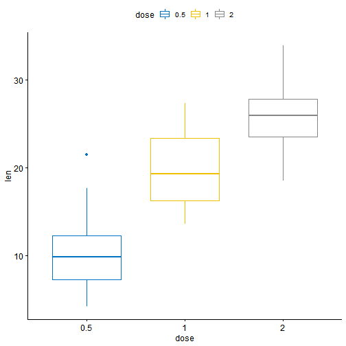
# Dot plot (dp)
dp <- ggdotplot(ToothGrowth, x = "dose", y = "len",
                 color = "dose", palette = "jco", binwidth = 1)
dp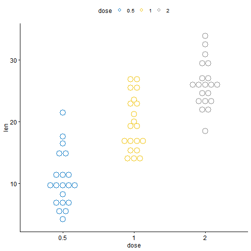
data("mtcars")
mtcars$name <- rownames(mtcars)
mtcars$cyl <- as.factor(mtcars$cyl)
head(mtcars[, c("name", "wt", "mpg", "cyl")])
## name wt mpg cyl
## Mazda RX4 Mazda RX4 2.62 21.0 6
## Mazda RX4 Wag Mazda RX4 Wag 2.88 21.0 6
## Datsun 710 Datsun 710 2.32 22.8 4
## Hornet 4 Drive Hornet 4 Drive 3.21 21.4 6
## Hornet Sportabout Hornet Sportabout 3.44 18.7 8
## Valiant Valiant 3.46 18.1 6# Bar plot (bp)
bp <- ggbarplot(mtcars, x = "name", y = "mpg",
fill = "cyl", # change fill color by cyl
color = "white", # Set bar border colors to white
palette = "jco", # jco journal color palett. see ?ggpar
sort.val = "asc", # Sort the value in ascending order
sort.by.groups = TRUE, # Sort inside each group
x.text.angle = 90 # Rotate vertically x axis texts
)
bp + font("x.text", size = 8)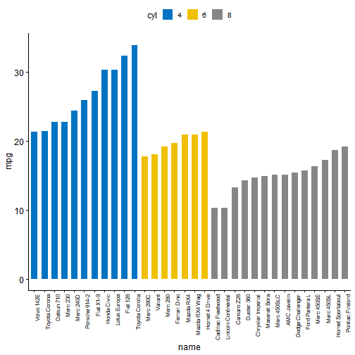
# Scatter plots (sp)
sp <- ggscatter(mtcars, x = "wt", y = "mpg",
                add = "reg.line",               # Add regression line
                conf.int = TRUE,                # Add confidence interval
                color = "cyl", palette = "jco", # Color by groups "cyl"
                shape = "cyl"                   # Change point shape by groups "cyl"
                )+
  stat_cor(aes(color = cyl), label.x = 3)       # Add correlation coefficient
sp
## `geom_smooth()` using formula 'y ~ x'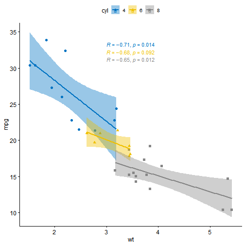
组合多张图片在一个面板上
使用 ggpubr包的 ggarrange()进行以下操作:
ggarrange(bxp, dp, bp + rremove("x.text"),
          labels = c("A", "B", "C"),
          ncol = 2, nrow = 2)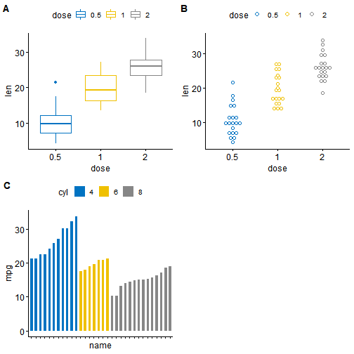
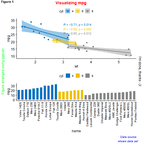
给图片添加注释
ggpubr包提供了函数 annotate_figure()可以对面板中图片整体或任意图片添加一定量的注释展示效果如下图:
figure <- ggarrange(sp, bp + font("x.text", size = 10),
                    ncol = 1, nrow = 2)
## `geom_smooth()` using formula 'y ~ x'annotate_figure(figure,
top = text_grob("Visualizing mpg", color = "red", face = "bold", size = 14),
bottom = text_grob("Data source: \n mtcars data set", color = "blue",
hjust = 1, x = 1, face = "italic", size = 10),
left = text_grob("Figure arranged using ggpubr", color = "green", rot = 90),
right = "I'm done, thanks :-)!",
fig.lab = "Figure 1", fig.lab.face = "bold"
)
图片对齐
最经典的例子就是在绘制生存曲线时,把risk table放在生存曲线图的下边。此时,我们需要调节表和图的大小和相对位置,使其分布更为合理
# Fit survival curves
library(survival)
fit <- survfit( Surv(time, status) ~ adhere, data = colon )
# Plot survival curves
library(survminer)
ggsurv <- ggsurvplot(fit, data = colon,
                     palette = "jco",                              # jco palette
                     pval = TRUE, pval.coord = c(500, 0.4),        # Add p-value
                     risk.table = TRUE                            # Add risk table
                     )
## Warning: Vectorized input to `element_text()` is not officially supported.
## Results may be unexpected or may change in future versions of ggplot2.ggarrange(ggsurv$plot, ggsurv$table, heights = c(2, 0.7),
ncol = 1, nrow = 2)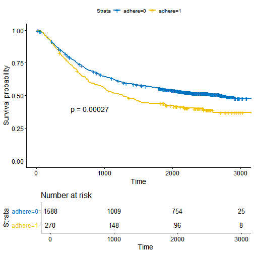
此时,我们可以看出图和表并不是完全垂直对齐的,要对齐他们需要调用 align参数
ggarrange(ggsurv$plot, ggsurv$table, heights = c(2, 0.7),
          ncol = 1, nrow = 2, align = "v")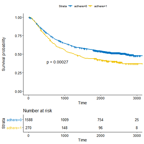
改变图形的行列布局排布
使用 ggpubr包
我们将使用嵌套的 ggarrange()函数来更改图的列/行跨度。
例如,我们使用下边的代码可以实现这样的布局
- 散点图(sp)将位于第一行并跨越两列
- 箱形图(bxp)和点图(dp)将首先排列,并且将在第二行中生活两列不同的列
ggarrange(sp,                                                 # First row with scatter plot
          ggarrange(bxp, dp, ncol = 2, labels = c("B", "C")), # Second row with box and dot plots
          nrow = 2,
          labels = "A"                                        # Labels of the scatter plot
          )
## `geom_smooth()` using formula 'y ~ x'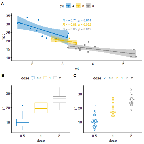
使用 cowplot包
函数 ggdraw()+ draw_plot()+ draw_plot_label()的组合可用于将图形放置在特定大小的特定位置。
ggdraw()可以初始化一个空的绘图画布,默认情况是这样的:

draw_plot()可以将绘图放置在绘图画布上的某处:
draw_plot(plot, x = 0, y = 0, width = 1, height = 1)draw_plot_label() 可以向图的左上角添加绘图标签。它可以处理带有关联坐标的标签向量。
draw_plot_label(label, x = 0, y = 1, size = 16, ...)如果需要组合多张图形,可以通过类似于下边的代码来实现:
library("cowplot")
ggdraw() +
  draw_plot(bxp, x = 0, y = .5, width = .5, height = .5) +
  draw_plot(dp, x = .5, y = .5, width = .5, height = .5) +
  draw_plot(bp, x = 0, y = 0, width = 1, height = 0.5) +
  draw_plot_label(label = c("A", "B", "C"), size = 15,
                  x = c(0, 0.5, 0), y = c(1, 1, 0.5))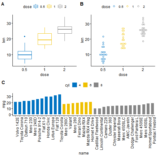
使用 gridExtra包
gridExtra包的使用方法和 ggpubr包类似
library("gridExtra")##
## Attaching package: 'gridExtra'## The following object is masked from 'package:dplyr':
##
## combinegrid.arrange(sp, # First row with one plot spaning over 2 columns
arrangeGrob(bxp, dp, ncol = 2), # Second row with 2 plots in 2 different columns
nrow = 2)## `geom_smooth()` using formula 'y ~ x'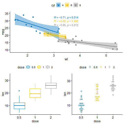
我们同样可以使用 gird.arrange()函数中的 lay_matrix参数来设置,使用方法如下:
grid.arrange(bp,                                    # bar plot spaning two columns
             bxp, sp,                               # box plot and scatter plot
             ncol = 2, nrow = 2,
             layout_matrix = rbind(c(1,1), c(2,3)))
## `geom_smooth()` using formula 'y ~ x'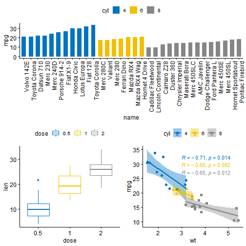
在上面的R代码中,layout_matrix是一个2×2矩阵(2列和2行)。 第一行全是1,这是第一幅图占的地方,横跨两列; 第二行包含分别占据一列的图2和图3
此时,如果需要对图形进行注释,ggpubr包已经不足以实现,需要我们使用 cowplot包来进行进一步的注释
需要注意的是 grid.arrange()/ arrangeGrob()输出的是一个 gtable,首先需要使用 ggpubr包中的 as_ggplot()函数将其转换为 ggplot。 接下来,就可以使用函数 draw_plot_label()对其进行注释。
library("gridExtra")
library("cowplot")
# Arrange plots using arrangeGrob
# returns a gtable (gt)
gt <- arrangeGrob(bp,                               # bar plot spaning two columns
             bxp, sp,                               # box plot and scatter plot
             ncol = 2, nrow = 2,
             layout_matrix = rbind(c(1,1), c(2,3)))
## `geom_smooth()` using formula 'y ~ x'# Add labels to the arranged plots
p <- as_ggplot(gt) + # transform to a ggplot
draw_plot_label(label = c("A", "B", "C"), size = 15,
x = c(0, 0, 0.5), y = c(1, 0.5, 0.5)) # Add labels
p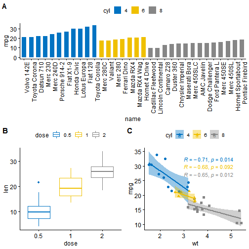
在上面的R代码中,我们使用了
arrangeGrob()而不是grid.arrange()。 请注意,这两个函数的主要区别在于,grid.arrange()会自动绘制排列好的图 由于我们要在绘制之前注释已排列的图,因此在这种情况下,函数arrangeGrob()是首选。
使用 grid包
通过函数 grid.layout(),可以使用 gridR包创建复杂的图像布局。 它还提供了函数 viewport()来定义布局上图像的区域或位置。 函数 print()用于将图放置在指定区域中。
总结起来共以下5个顺序步骤:
- 创建绘图:p1,p2,p3,…
- 使用函数
grid.newpage()创建画板 - 创建画板布局2X2 - 列数= 2; 行数= 2
- 定义图像输出位置:画板中图像显示的区域
- 在画板中输出显示图片
library(grid)
# Move to a new page
grid.newpage()
# Create layout : nrow = 3, ncol = 2
pushViewport(viewport(layout = grid.layout(nrow = 3, ncol = 2)))
# A helper function to define a region on the layout
define_region <- function(row, col){
  viewport(layout.pos.row = row, layout.pos.col = col)
}
# Arrange the plots
print(sp, vp = define_region(row = 1, col = 1:2))   # Span over two columns
## `geom_smooth()` using formula 'y ~ x'print(bxp, vp = define_region(row = 2, col = 1))
print(dp, vp = define_region(row = 2, col = 2))
print(bp + rremove("x.text"), vp = define_region(row = 3, col = 1:2))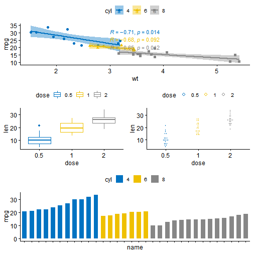
通用图例的设定
在我们绘制的图片当中,有的可能具有相同的图例,函数 ggarrange()可以与以下参数一起使用,使两幅图使用相同的图例
common.legend = TRUE:使用公共图例legend:指定图例位置。 允许的值包括c(“top”,“bottom”,“left”,“right”)
ggarrange(bxp, dp, labels = c("A", "B"),
          common.legend = TRUE, legend = "bottom")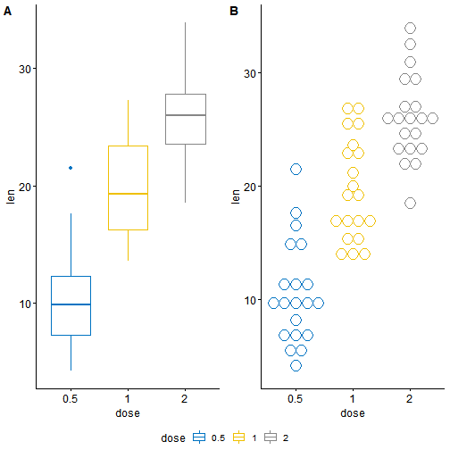
实战
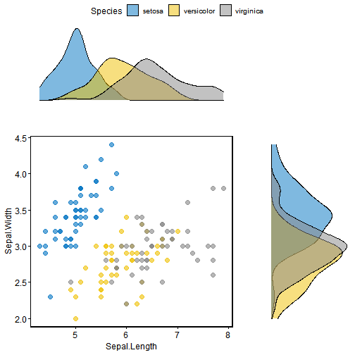
给散点图添加边界密度图
# Scatter plot colored by groups ("Species")
sp <- ggscatter(iris, x = "Sepal.Length", y = "Sepal.Width",
                color = "Species", palette = "jco",
                size = 3, alpha = 0.6)+
  border()
# Marginal density plot of x (top panel) and y (right panel)
xplot <- ggdensity(iris, "Sepal.Length", fill = "Species",
                   palette = "jco")
yplot <- ggdensity(iris, "Sepal.Width", fill = "Species",
                   palette = "jco")+
  rotate()
# Cleaning the plots
yplot <- yplot + clean_theme()
xplot <- xplot + clean_theme()
# Arranging the plot
ggarrange(xplot, NULL, sp, yplot,
          ncol = 2, nrow = 2,  align = "hv",
          widths = c(2, 1), heights = c(1, 2),
          common.legend = TRUE)