bioinfo

无监督聚类分析流程

Jeason

2726字约9分钟

biosoftwareclustering

2025-7-17

无监督类别发现是一种数据挖掘方法，它仅基于内在特征而不依赖外部变量来识别未知的可能项目组（聚类）。聚类基本上包括四个步骤：

数据准备
Dissimilarity矩阵计算
聚类
评估聚类分配

数据准备

在此步骤中，我们需要过滤掉不完整的病例和低表达基因，然后对基因表达值进行转换/归一化。通常，分析从 RNA 测序实验的原始计数矩阵开始。我保留了在 10% 的样本中表达且计数为 10 或更高的基因。所有缺失值都必须删除，或者如果要保留它们，则需要估算它们的值。在我的数据集中，没有缺失值。对于转换/归一化，我使用方差稳定变换 (VST)，该变换是 DESeq2 packages 中实现的 vst 函数，它同时还会对原始计数进行归一化。使用其他类型的变换（例如 Z 值和对数变换）也很常见。如果表达矩阵包含估计的转录本计数（例如 RSEM）或根据测序深度归一化的计数（例如 FPKM），则对这些值进行 log2 变换将为聚类做好准备。请参考以下示例：

使用 log2(RSEM)基因表达值，去除样本间 NA 值超过 10%的基因。然后根据样本间基因表达的标准差，选出变异最大的前 25%的基因（A. Gordon Robertson et al., Cell,2017）
使用 FPKM 矩阵并在至少 10% 的样本中保留具有 log2(FPKM+1)>2 的基因，并选择 MAD 排序基因的子集 (2K, 4K, 6K) 来识别稳定的类别（Jakob Hedegaard et al, Cancer Cell, 2016）

特征选择：由于表达矩阵中存在大量特征（基因），因此应进行特征选择步骤，从而将分析范围限制在那些可能解释队列样本间差异的基因上。因此，建议选择用于后续聚类的特征。我根据中位绝对偏差 (MAD) 选择了排名靠前的 2k、4k 和 6k 个基因。还可以应用许多其他方法，例如“基于最大方差的特征选择”、“基于主成分分析 (PCA) 的特征降维和提取”以及“基于 Cox 回归模型的特征选择”。更多信息，请参阅 Bioconductor 软件包 CancerSubtypes 手册。

#_________________________________reading data and processing_________________________________#
# reading count data
rna <- read.table("Uromol1_CountData.v1.csv", header = T, sep = ",", row.names = 1)
head(rna[1:5, 1:5], 5)
#                   U0001 U0002 U0006 U0007 U0010
#ENSG00000000003.13  1458   228  1800  3945   293
#ENSG00000000005.5      0     0     9     0     0
#ENSG00000000419.11   594    23   792  1378   139
#ENSG00000000457.12   548    22  1029   976   148
#ENSG00000000460.15    53     2   190   136    47

dim(rna)
# [1] 60483   476  This is a typical output from hts-seq count matrix with more than 60,000 genes

# Dissecting dataset based on gene-type
library(biomaRt)
mart <- useDataset("hsapiens_gene_ensembl", useMart("ensembl"))
genes <- getBM(attributes= c("ensembl_gene_id","hgnc_symbol", "gene_biotype"), 
               mart= mart)

# see gene types returned by biomaRt
data.frame(table(genes$gene_biotype))[order(- data.frame(table(genes$gene_biotype))[,2]), ]

# We will continue with protein-coding here:
rna <- rna[substr(rownames(rna),1,15) %in% genes$ensembl_gene_id[genes$gene_biotype == "protein_coding"],]

dim(rna)
#[1] 19581   476 These are protein-coding genes

# Reading associated clinical data
clinical.exp <- read.table("uromol_clinic.csv", sep = ",", header = T, row.names = 1)
head(clinical.exp[1:5,1:5], 5)
#      UniqueID   CLASS  BASE47    CIS X12.gene.signature
#U0603    U0603 luminal luminal no-CIS          high_risk
#U0497    U0497 luminal   basal no-CIS           low_risk
#U0839    U0839 luminal luminal    CIS           low_risk
#U1043    U1043 luminal luminal no-CIS          high_risk
#U0566    U0566 luminal   basal no-CIS           low_risk

# Make sure about sample order in rna and clincal.exp dataset
all(rownames(clinical.exp) %in% colnames(rna))
#[1] TRUE
all(rownames(clinical.exp) == colnames(rna))
#[1] FALSE
# reordering rna dataset
rna <- rna[, rownames(clinical.exp)]
#______________________ Data transformation & Normalization ______________________________#
library(DESeq2)
dds <- DESeqDataSetFromMatrix(countData = rna,
                              colData = clinical.exp,
                              design = ~ 1) # 1 passed to the function because of no model
# pre-filteration, however while using DESeq2 package it is not necessary, because the function automatically will filter out low-count genes
# Keeping genes with expression in 10% of samples with a count of 10 or higher
keep <- rowSums(counts(dds) >= 10) >= round(ncol(rna)*0.1)
dds <- dds[keep,]

# vst transformation
vsd <- assay(vst(dds)) # For a fully unsupervised transformation one can set blind = TRUE (which is the default).
#_________________________________# Feature Selection _________________________________#
# top 5K based on MAD 

mads=apply(vsd,1,mad)
# check data distribution
hist(mads, breaks=nrow(vsd)*0.1)
# selecting features
mad2k=vsd[rev(order(mads))[1:2000],]
#mad4k=vsd[rev(order(mads))[1:4000],]
#mad6k=vsd[rev(order(mads))[1:6000],]

Dissimilarity矩阵计算

聚类是将相似的样本分到一个聚类中，并根据距离度量将它们与不相似的样本区分开来。相异度矩阵的计算方法（距离度量）有很多种。要查看可用的距离度量列表，请查看 ?stats::dist 和 ?vegan::vegdist()

对于log-transformed gene expression，可以应用基于欧几里得(Euclidean)的测量方法。
对于 RNA-seq normalized counts，可以使用基于相关性的测量（Pearson、Spearman）或基于泊松的距离。

聚类

大部分的聚类算法可以通过diceR包来实现。最广泛使用的算法是划分聚类(partitional clustering)和层次聚类(hierarchical clustering) 。

划分聚类是一种根据样本的相似性将样本划分为多个聚类的方法。算法需要指定要生成的聚类数量。常用的划分聚类包括：

K-means聚类：每个聚类由属于该聚类的数据点的中心或均值表示。此方法对异常值敏感。
K-中心点聚类（K-medoids clustering）或 PAM（Partitioning Around Medoids）：其中每个聚类由该聚类中的一个对象表示。PAM 对异常值不太敏感。

层次聚类与划分聚类相比，此方法不需要预先指定要生成的聚类数量。HC 可分为两类：

凝聚（Agglomerative）：bottom-up的方法，每个观察最初被视为其自己的一个聚类（叶子），并且随着聚类在层次结构中向上移动，聚类对会合并。
分裂（Divisive）：top-down的方法，从根开始，因此所有观察都从一个集群开始，并且随着层次结构的向下移动，分裂以递归方式执行。

关于如何计算聚类间距离的一些说明：实际上，存在多种进行聚类聚集（即链接）的方法。使用 stat 包时，可能的方法包括ward.D、ward.D2、single、complete、average、mcquitty、median或centroid。通常，首选complete和Ward法。更多相关阅读材料可在link找到。因此，层次聚类提供了一种基于树的对象表示，也称为树状图。

在实践中，HC、KM 和 PAM 通常用于基因表达数据。为了定量确定数据集中可能聚类的数量和成员资格，我将使用共识聚类 (CC) 方法。

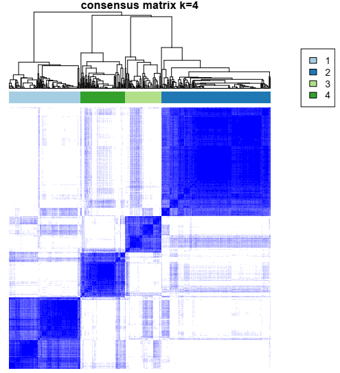
要根据 CC 确定聚类数量，有几种图形可以提供帮助。（1）对应于共识矩阵的彩色热图，代表从 0 到 1 的共识值；白色对应 0（从不聚集在一起），深蓝色对应 1（始终聚集在一起）。（2）共识累积分布函数 (CDF) 图，该图可让人确定在聚类数量 k 为多少时，CDF 达到近似最大值。因此，共识和聚类置信度在此 k 处达到最大值。（3）基于 CDF 图，可以绘制 CDF 曲线下面积相对变化的图表。该图允许用户确定共识的相对增加，并确定没有明显增加的 k。

#_________________________________# Clustering & Cluster assignment validation _________________________________#
# Finding optimal clusters by CC
library(ConsensusClusterPlus)
results = ConsensusClusterPlus(mad2k,
                               maxK=6,
                               reps=50,
                               pItem=0.8,
                               pFeature=1,
                               title= "geneExp",
                               clusterAlg="pam",
                               distance="spearman",
                               seed=1262118388.71279,
                               plot="pdf")

在本文中，我选择了 80% 的项目重采样 ( pItem ) 和 80% 的基因重采样 ( pFeature )，并将最大评估 k 设为 6，以便评估聚类计数 ( maxK ) 分别为 2、3、4、5、6，重采样次数 ( reps ) 为 50 次，基于中心点算法 ( clusterAlg ) 的分区以及 Spearman 相关距离 ( distance )，为输出添加了标题 ( title )，并要求将图形结果写入 PDF plot 文件。我还设置了一个随机种子，以便此示例可重复使用 ( seed )。

上述命令返回几个图，有助于决定聚类数量，特别是显示一致性 CDF 和 CDF 曲线下面积相对变化的图。

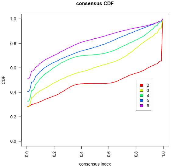
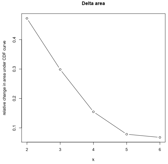
因此，通过查看图表，在这种情况下，最佳聚类数量应为四个。下图是 k = 4 时样本的一致性图。其他 k 值的结果可在结果 PDF 文件中找到。

评估聚类分配

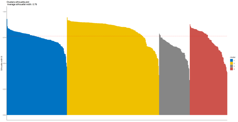
评估聚类分配或聚类验证是指评估聚类结果优劣的过程。Alboukadel Kassambara 发表了一篇关于此主题的详细文章。在本教程中，我将使用 Silhouette 方法进行聚类评估。此方法可用于研究所得聚类之间的分离距离。Silhouette 图反映了一个聚类中每个数据点与相邻聚类中某个点的接近程度。该度量（Silhouette 宽度）的范围为 -1 到 +1。接近 +1 的值表示样本距离相邻聚类中最近的数据点较远。负值可能表示聚类分配错误，接近 0 的值则表示对该数据点的聚类分配是任意的。

因为通过聚类，人们应该期望找到在生存概率方面有显著差异的样本聚类，所以作为从生物学角度评估聚类分配的一种方式，我在聚类（亚型）之间进行生存分析，以查看是否存在显著差异。

ConsensusClusterPlus 的输出是一个列表，对于每个 k 值（例如 k = 4），可以通过 results[[4]] 访问。我将结果保存在一个新对象中，然后继续计算并绘制轮廓图。

#_________________________________#Assessing cluster assignment _________________________________#
#Silhouette width analysis
cc4 = results[[4]]

# calcultaing Silhouette width using the cluster package 
library(cluster)
cc4Sil = silhouette(x = cc4[[3]], # x is a numeric vector that indicates cluster assignment for each data point
                    dist = as.matrix(1- cc4[[4]])) # dist should be a distance matrix and NOT a similarity matrix, so I subtract the matrix from one to get that dist matrix

#For visualization:
library(factoextra)
fviz_silhouette(cc4Sil, palette = "jco",
                 ggtheme = theme_classic())

上述函数返回每个聚类的轮廓宽度的摘要：

  cluster size ave.sil.width
1       1  130          0.75
2       2  199          0.83
3       3   66          0.65
4       4   81          0.72

从下图中，我们可以了解平均 Silhoutte 宽度以及每个簇的大小。

#_________________________________#Assessing cluster assignment _________________________________#
#Survival analysis
### Preparing dataset for survival analysis
cc4Class = data.frame(cc4$consensusClass)
cc4Class$ID = rownames(cc4Class)
cc4Class = data.frame(cc4Class[match(rownames(clinical.exp),cc4Class$ID),])
all(cc4Class$ID == rownames(clinical.exp))

# new encoding for status, time, and cluster
clinical.exp$status = ifelse(clinical.exp$Progression.to.T2. == "NO", 0,1)
clinical.exp$time = as.numeric(clinical.exp$Progression.free.survival..months. * 30)
clinical.exp$cluster = as.factor(cc4Class$cc4.consensusClass)

library(survival)

res.cox <- coxph(Surv(time, status) ~ cluster, data = clinical.exp)
res.cox

Call:
coxph(formula = Surv(time, status) ~ cluster, data = clinical.exp)

             coef exp(coef) se(coef)      z       p
cluster2 -1.47638   0.22846  0.48357 -3.053 0.00226
cluster3  0.22532   1.25272  0.42213  0.534 0.59351
cluster4 -2.39949   0.09076  1.03301 -2.323 0.02019

Likelihood ratio test=21.88  on 3 df, p=6.908e-05
n= 476, number of events= 31

summary(res.cox)

Call:
coxph(formula = Surv(time, status) ~ cluster, data = clinical.exp)

  n= 476, number of events= 31 

             coef exp(coef) se(coef)      z Pr(>|z|)   
cluster2 -1.47638   0.22846  0.48357 -3.053  0.00226 **
cluster3  0.22532   1.25272  0.42213  0.534  0.59351   
cluster4 -2.39949   0.09076  1.03301 -2.323  0.02019 * 
---
Signif. codes:  0 ‘***’ 0.001 ‘**’ 0.01 ‘*’ 0.05 ‘.’ 0.1 ‘ ’ 1

         exp(coef) exp(-coef) lower .95 upper .95
cluster2   0.22846     4.3771   0.08855    0.5894
cluster3   1.25272     0.7983   0.54769    2.8653
cluster4   0.09076    11.0175   0.01198    0.6874

Concordance= 0.714  (se = 0.039 )
Likelihood ratio test= 21.88  on 3 df,   p=7e-05
Wald test            = 16.52  on 3 df,   p=9e-04
Score (logrank) test = 22.14  on 3 df,   p=6e-05

译文来源：https://github.com/hamidghaedi/Unsupervised_Clustering_for_Gene_Expression_data